Analytic diffusion
examples/analytic_diffusion.py models a diffusion process and reports the error from the model integration by comparison to the analytic solution (intial concentrations are taken from Green’s function expressions for respective geometry).
$ python analytic_diffusion.py --help
usage: analytic_diffusion.py [-h] [-D D] [--t0 T0] [--tend TEND] [--x0 X0]
                             [--xend XEND] [--mu MU] [-N N] [--nt NT]
                             [-g GEOM] [--logt] [--logy] [--logx] [--random]
                             [-k K] [--nstencil NSTENCIL] [--linterpol]
                             [--rinterpol] [--num-jacobian] [--method METHOD]
                             [-p] [-a ATOL] [--rtol RTOL] [-e]
                             [--random-seed RANDOM_SEED] [-s SAVEFIG] [-v]

optional arguments:
  -h, --help            show this help message and exit
  -D D, --D D           0.002
  --t0 T0               3.0
  --tend TEND           7.0
  --x0 X0               0.0
  --xend XEND           1.0
  --mu MU               -
  -N N, --N N           64
  --nt NT               42
  -g GEOM, --geom GEOM  u'f'
  --logt                False
  --logy                False
  --logx                False
  --random              False
  -k K, --k K           0.0
  --nstencil NSTENCIL   3
  --linterpol           False
  --rinterpol           False
  --num-jacobian        False
  --method METHOD       u'bdf'
  -p, --plot            False
  -a ATOL, --atol ATOL  1e-06
  --rtol RTOL           1e-06
  -e, --efield          False
  --random-seed RANDOM_SEED
                        42
  -s SAVEFIG, --savefig SAVEFIG
                        u'None'
  -v, --verbose         False
$ python analytic_diffusion.py --plot --efield --mu 0.5 --nstencil 5 --k 0.1 --geom f

$ python analytic_diffusion.py --x0 0 --xend 1000 --N 1000 --mu 500 -D 400 --nstencil 3
Note -D 475
$ python analytic_diffusion.py --x0 0 --xend 1000 --N 1000 --mu 500 -D 475 --nstencil 7
Still problematic (should not need to be):
$ python analytic_diffusion.py --plot --nstencil 5 --logy --D 0.0005
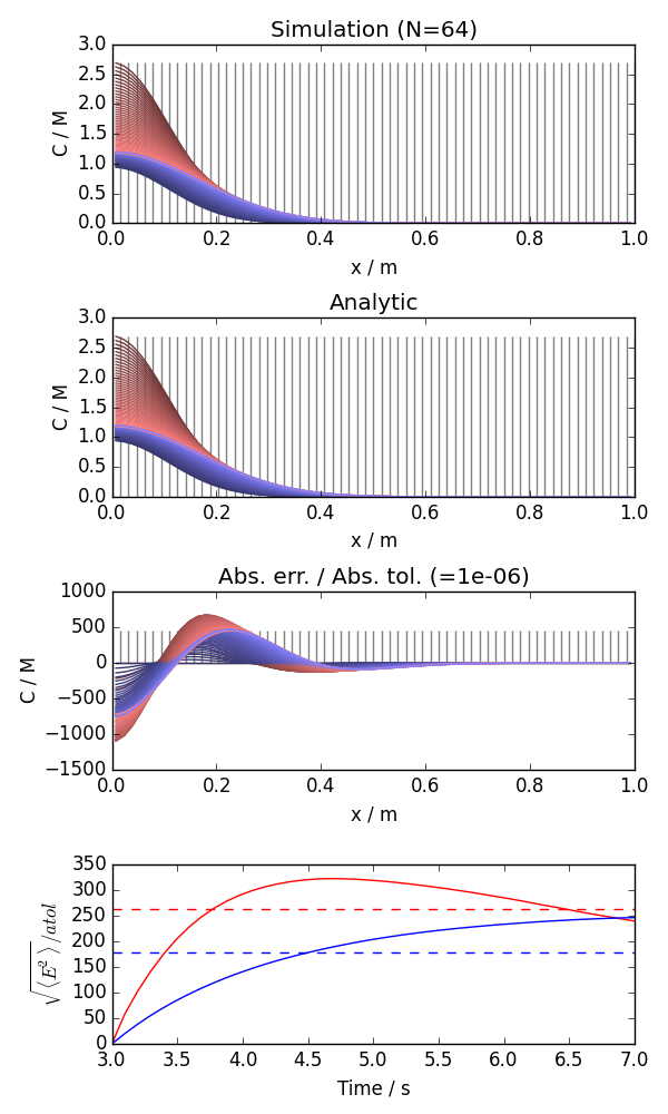
Here is an example generated by:
$ python analytic_diffusion.py --plot --nstencil 3 --k 0.1 --geom f --savefig analytic_diffusion.png
- analytic_diffusion.cylindrical_analytic(x, t, D, mu, x0, xend, v, logy=False, logx=False)[source]
Evaluates the Green’s function:
\[c(x, t) = \frac{x_{end}-x_{0}}{4 \pi D t} \ e^{-\frac{(x - \mu - vt)^2}{4Dt}}\]which satisfies:
\[\frac{\partial c(x, t)}{\partial t} = D\nabla^2 \ c(x, t) - \vec{v} \cdot c(x, t)\]where \(\nabla\) in cylindrical coordinates with axial symmetry is:
\[\nabla = \frac{1}{x}\]and where \(\nabla^2\) is:
\[\nabla^2 = \frac{1}{x} \frac{\partial}{\partial x} \left( x \frac{\partial}{\partial x} \right)\]
- analytic_diffusion.flat_analytic(x, t, D, mu, x0, xend, v, logy=False, logx=False)[source]
Evaluates the Green’s function:
\[c(x, t) = \frac{x_{end}-x_{0}}{\sqrt{4 \pi D t}} \ e^{-\frac{(x - \mu - vt)^2}{4Dt}}\]which satisfies:
\[\frac{\partial c(x, t)}{\partial t} = D\nabla^2 \ c(x, t) - \vec{v} \cdot c(x, t)\]where \(\nabla\) in cartesian coordinates with planar (yz-plane) symmetry is:
\[\nabla = \frac{\partial}{\partial x}\]and where \(\nabla^2\) :
\[\nabla^2 = \frac{\partial^2}{\partial x^2}\]
- analytic_diffusion.integrate_rd(D=0.002, t0=3.0, tend=7.0, x0=0.0, xend=1.0, mu=None, N=64, nt=42, geom=u'f', logt=False, logy=False, logx=False, random=False, k=0.0, nstencil=3, linterpol=False, rinterpol=False, num_jacobian=False, method=u'bdf', plot=False, atol=1e-06, rtol=1e-06, efield=False, random_seed=42, savefig=u'None', verbose=False)[source]
- analytic_diffusion.spherical_analytic(x, t, D, mu, x0, xend, v, logy=False, logx=False)[source]
Evaluates the Green’s function:
\[c(x, t) = \frac{x_{end}-x_{0}}{\sqrt{4 \pi D t^3}} \ e^{-\frac{(x - \mu - vt)^2}{4Dt}}\]which satisfies:
\[\frac{\partial c(x, t)}{\partial t} = D\nabla^2 c(x, t) - \vec{v} \cdot c(x, t)\]where \(\nabla\) in spherical coordinates for a isotropic system is:
\[\nabla = \frac{\partial}{\partial x}\]and where \(\nabla^2\) is:
\[\nabla^2 = \frac{1}{x^2} \frac{\partial}{\partial x} \left( x^2 \frac{\partial}{\partial x} \right)\]