Two coupled decays

examples/decay.py demonstrates accuracy by comparison with analytic solution for a simple system of two coupled decays

$ python decay.py --help

usage: decay.py [-h] [--tend TEND] [-A A0] [--nt NT] [--t0 T0] [--rates RATES]
                [--logy] [--logt] [--plot] [--savefig SAVEFIG] [-m METHOD]
                [-a ATOL] [--rtol RTOL] [--num-jac] [--scale-err SCALE_ERR]
                [--small SMALL] [--plotlogy] [--plotlogt] [-v]

    Analytic solution through Bateman equation =>
    ensure :math:`|k_i - k_j| \gg eps`


optional arguments:
  -h, --help            show this help message and exit
  --tend TEND           2.0
  -A A0, --A0 A0        1.0
  --nt NT               67
  --t0 T0               0.0
  --rates RATES         u'3.40715,4.0'
  --logy                False
  --logt                False
  --plot                False
  --savefig SAVEFIG     u'None'
  -m METHOD, --method METHOD
                        u'bdf'
  -a ATOL, --atol ATOL  u'1e-7,1e-6,1e-5'
  --rtol RTOL           u'1e-6'
  --num-jac             False
  --scale-err SCALE_ERR
                        1.0
  --small SMALL         u'None'
  --plotlogy            False
  --plotlogt            False
  -v, --verbose         False

Here is an example generated by:

$ python decay.py --plot --savefig decay.png

decay.get_Cref(k, y0, tout)

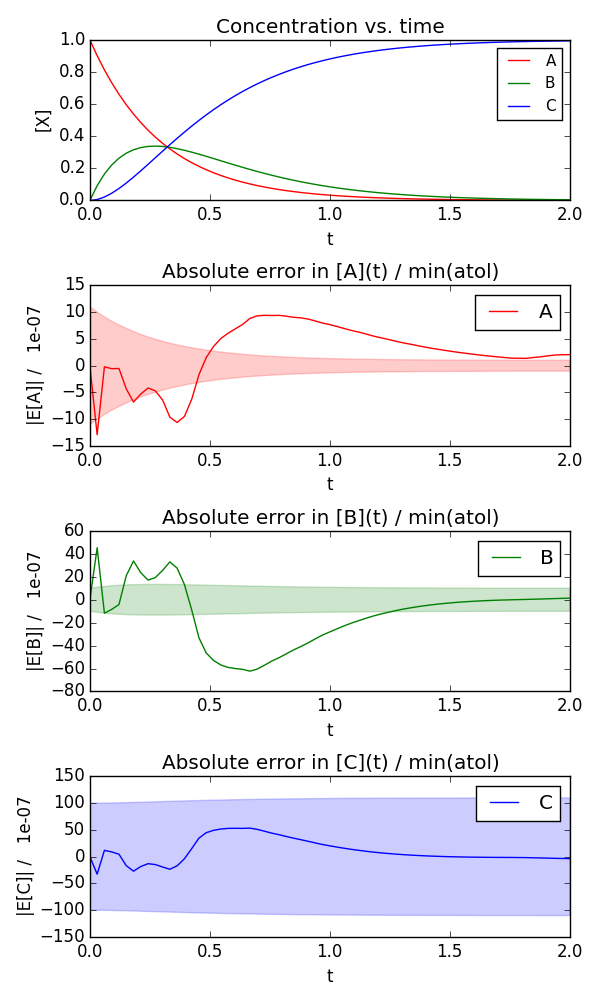
decay.integrate_rd(tend=2.0, A0=1.0, nt=67, t0=0.0, rates=u'3.40715, 4.0', logy=False, logt=False, plot=False, savefig=u'None', method=u'bdf', atol=u'1e-7, 1e-6, 1e-5', rtol=u'1e-6', num_jac=False, scale_err=1.0, small=u'None', plotlogy=False, plotlogt=False, verbose=False)

Analytic solution through Bateman equation => ensure \(|k_i - k_j| \gg eps\)