Steady state approximation

examples/steady_state_approx.py shows how you can estimate errors commited when assuming steady state for simple systems. In this essence it is quite different from the other examples where we have been investigating the error of the numerical integration vs. an analytic solution. Here we will do the reverse, we will assume that our result from the numerical integration is correct (or rather: much more accurate) compared to our approximately correct analytic expressions.

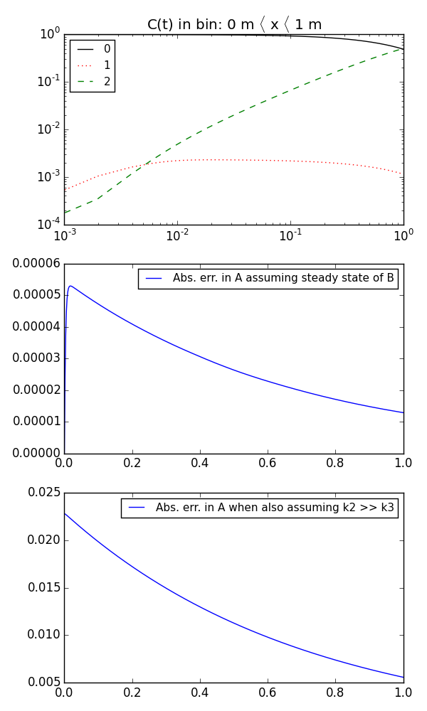
We will consider the following system:

\[\begin{split}A & &\rightarrow B & &~~~k_1 \\ & B &\rightarrow C & &~~~k_2 \\ A + &B &\rightarrow B &+ C &~~~k_3\end{split}\]

\[\begin{split}\frac{dA}{dt} &= -k1 \cdot A & &- k3 \cdot A \cdot B \\ \frac{dB}{dt} &= +k1 \cdot A &- k2 \cdot B & \\ \frac{dC}{dt} &= &+ k2 \cdot B &+ k3 \cdot A \cdot B\end{split}\]

The rate expressions are from mass action and hence we are conserving mass:

\[A+B+C = A_0 + B_0 + C_0\]

sum of derivatives = 0 (already satisfied)

For initial concentrations of A much larger than B we have:

Steady state assumption for B (\(A_0 \gg B_0\)):

\[\begin{split}B &= \frac{k_1 A}{k_2} \\ \frac{dA}{dt} &= -k_1\left(A + \frac{k_3}{k_2}A^2 \right) \\ \log{A} - \log{\left( \frac{k_3}{k_2}A + 1 \right)} &= -k_1t + \left(\log{A_0} - \log{\left( \frac{k_3}{k_2}A_0 + 1\right)}\right) \\ \frac{A}{\frac{k_3}{k_2}A + 1} &= f(t)\end{split}\]

using

\[f(t) = \frac{A_0}{\frac{k_3}{k_2}A_0 + 1}e^{-k_1 t}\]

we get

\[\begin{split}A(1 - f(t) \cdot \frac{k_3}{k_2}) &= f(t) \\ A &= \frac{f(t)}{1 - f(t)\frac{k_3}{k_2}} [*] \\ A &= \frac{1}{\frac{1}{f(t)} - \frac{k_3}{k_2}} \\ A &= \frac{1}{\frac{\frac{k_3}{k_2}A_0 + 1}{A_0}e^{k_1 t} - \frac{k_3}{k_2}} \\\end{split}\]

where we note:

\[\begin{split}[*] ~~ if \frac{k_3}{k_2} << 1: \\ A = f(t)\end{split}\]

steady_state_approx.integrate_rd(tend=1.0, k1=0.7, k2=300.0, k3=7.0, A0=1.0, B0=0.0, C0=0.0, nt=512, plot=False, savefig=u'None')

Runs integration and (optionally) generates plots.

Examples

$ python steady_state_approx.py --plot --savefig steady_state_approx.png

$ python steady_state_approx.py --plot --savefig steady_state_approx.html

steady_state_approx.html