Diffusion from constant concentration surface

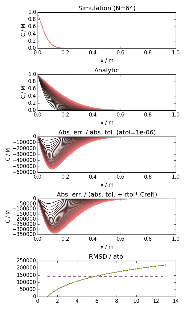
examples/const_surf_conc.py models a diffusion process and reports the error from the model integration by comparison to the analytic solution (intial concentrations are taken from Green’s function expressions for respective geometry).

$ python const_surf_conc.py --help

usage: const_surf_conc.py [-h] [-D D] [--t0 T0] [--tend TEND] [--x0 X0]
                          [--xend XEND] [-N N] [--nt NT] [--logt] [--logy]
                          [--logx] [--random] [-k K] [--nstencil NSTENCIL]
                          [--linterpol] [--rinterpol] [--num-jacobian]
                          [-m METHOD] [-p] [-a ATOL] [--rtol RTOL] [-f FACTOR]
                          [--random-seed RANDOM_SEED] [--savefig SAVEFIG] [-v]
                          [--scaling SCALING]

    Solves the time evolution of diffusion from a constant source term.
    Optionally plots the results. In the plots time is represented by
    color scaling from black (:math:`t_0`) to red (:math:`t_{end}`)


optional arguments:
  -h, --help            show this help message and exit
  -D D, --D D           0.002
  --t0 T0               1.0
  --tend TEND           13.0
  --x0 X0               1e-10
  --xend XEND           1.0
  -N N, --N N           64
  --nt NT               42
  --logt                False
  --logy                False
  --logx                False
  --random              False
  -k K, --k K           1.0
  --nstencil NSTENCIL   3
  --linterpol           False
  --rinterpol           False
  --num-jacobian        False
  -m METHOD, --method METHOD
                        u'bdf'
  -p, --plot            False
  -a ATOL, --atol ATOL  1e-06
  --rtol RTOL           1e-06
  -f FACTOR, --factor FACTOR
                        100000.0
  --random-seed RANDOM_SEED
                        42
  --savefig SAVEFIG     u'None'
  -v, --verbose         False
  --scaling SCALING     1.0

Here is an example generated by:

$ python const_surf_conc.py --plot --savefig const_surf_conc.png

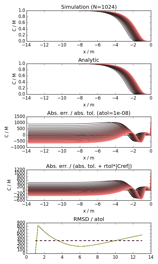
Solving the transformed system (\(\frac{d}{dt} \ln(c(\ln(x), t))\)):

$ python const_surf_conc.py --plot --N 1024 --verbose --nstencil 3 --scaling 1e-20 --logx --logy --factor 1e12 --x0 1e-6 --atol 1e-8 --rtol 1e-8 --savefig const_surf_conc_logy_logx.png

const_surf_conc.analytic(x, t, D, x0, xend, logx=False, c_s=1)

Evaluates the analytic expression for the concentration in a medium with a constant source term at x=0:

\[c(x, t) = c_s \mathrm{erfc}\left( \frac{x}{2\sqrt{Dt}}\right)\]

where \(c_s\) is the constant surface concentration.

const_surf_conc.integrate_rd(D=0.002, t0=1.0, tend=13.0, x0=1e-10, xend=1.0, N=64, nt=42, logt=False, logy=False, logx=False, random=False, k=1.0, nstencil=3, linterpol=False, rinterpol=False, num_jacobian=False, method=u'bdf', plot=False, atol=1e-06, rtol=1e-06, factor=100000.0, random_seed=42, savefig=u'None', verbose=False, scaling=1.0)

Solves the time evolution of diffusion from a constant source term. Optionally plots the results. In the plots time is represented by color scaling from black (\(t_0\)) to red (\(t_{end}\))