Equilibrium¶

examples/equilibrium.py demonstrates how scaling can be used together with tolerances to achieve desired accuracy from the numerical integration.

We will consider the transient towards an equilibrium for a dimerization:

\[\begin{split}A + &B &\overset{k_f}{\underset{k_b}{\rightleftharpoons}} C\end{split}\]

The analytic solution is (its derivation is left as an exercise):

\[\begin{split}A(t) &= A_0 - x(t) \\ B(t) &= B_0 - x(t) \\ C(t) &= C_0 + x(t) \\ x(t) &= \frac{(U-b)(U+b)(e^{Ut}-1)}{2k_f(Ue^{Ut} + U - qe^{Ut} + q)} \\\end{split}\]

where

\[\begin{split}U &= \sqrt{A^2k_f^2 + 2ABk_f^2 - 2Ak_bk_f + B^2k_f^2 - 2Bk_bk_f + 4Ck_bk_f + k_b^2} \\ q &= Ak_f + Bk_f - k_b\end{split}\]

$ python equilibrium.py --help

usage: equilibrium.py [-h] [--tend TEND] [-A A0] [-B B0] [-C C0] [--nt NT]
                      [--t0 T0] [--kf KF] [--kb KB] [-a ATOL] [-r RTOL]
                      [--logy] [--logt] [--num-jac] [--plot]
                      [--savefig SAVEFIG] [--splitplots] [--plotlogy]
                      [--plotsymlogy] [--plotlogt] [--scale-err SCALE_ERR]
                      [--scaling SCALING] [-v]

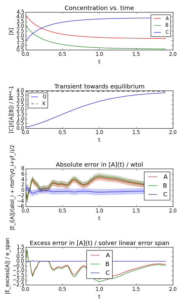
    Runs the integration and (optionally) plots:

    - Individual concentrations as function of time
    - Reaction Quotient vs. time (with equilibrium constant as reference)
    - Numerical error commited (with tolerance span plotted)
    - Excess error committed (deviation outside tolerance span)

    Concentrations (A0, B0, C0) are taken to be in "M" (molar),
    kf in "M**-1 s**-1" and kb in "s**-1", t0 and tend in "s"


optional arguments:
  -h, --help            show this help message and exit
  --tend TEND           1.9
  -A A0, --A0 A0        4.2
  -B B0, --B0 B0        3.1
  -C C0, --C0 C0        1.4
  --nt NT               100
  --t0 T0               0.0
  --kf KF               0.9
  --kb KB               0.23
  -a ATOL, --atol ATOL  u'1e-7,1e-6,1e-5'
  -r RTOL, --rtol RTOL  u'1e-6'
  --logy                False
  --logt                False
  --num-jac             False
  --plot                False
  --savefig SAVEFIG     u'None'
  --splitplots          False
  --plotlogy            False
  --plotsymlogy         False
  --plotlogt            False
  --scale-err SCALE_ERR
                        1.0
  --scaling SCALING     1.0
  -v, --verbose         False

Here is an example generated by:

$ python equilibrium.py --plot --savefig equilibrium.png

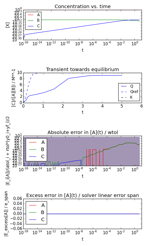
If concentrations are far from 1 (and below abstol) the accuracy of the numerical solution will be very poor:

$ python equilibrium.py --A0 1.0 --B0 1e-10 --C0 1e-30 --kf 10 --kb 1 --t0 0 --tend 5 --plot --plotlogy --plotlogt --savefig equilibrium_unscaled.png

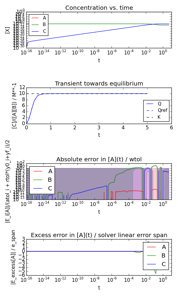
But by scaling the concentrations so that the smallest is well above the absolute tolerance we can get accurate results:

$ python equilibrium.py --scaling 1e10 --A0 1.0 --B0 1e-10 --C0 1e-30 --kf 10 --kb 1 --t0 0 --tend 5 --plot --plotlogy --plotlogt --savefig equilibrium_scaled.png

equilibrium.analytic_x(t, A, B, C, kf, kb, _exp=<ufunc 'exp'>)[source]¶

Analytic solution to the dimeriztion reaction:: A + B <=> C; (K = kf/kb)

equilibrium.integrate_rd(tend=1.9, A0=4.2, B0=3.1, C0=1.4, nt=100, t0=0.0, kf=0.9, kb=0.23, atol=u'1e-7, 1e-6, 1e-5', rtol=u'1e-6', logy=False, logt=False, num_jac=False, plot=False, savefig=u'None', splitplots=False, plotlogy=False, plotsymlogy=False, plotlogt=False, scale_err=1.0, scaling=1.0, verbose=False)[source]¶

Runs the integration and (optionally) plots:

Individual concentrations as function of time
Reaction Quotient vs. time (with equilibrium constant as reference)
Numerical error commited (with tolerance span plotted)
Excess error committed (deviation outside tolerance span)

Concentrations (A0, B0, C0) are taken to be in “M” (molar), kf in “M**-1 s**-1” and kb in “s**-1”, t0 and tend in “s”